论文复现 - Revisiting Weak-to-Strong Consistency in Semi-Supervised Semantic Segmentation

前记：这篇文章基于20年半监督学习的SOTA：FixMatch。他们发现FixMatch可以在半监督语义分割任务上媲美最近的SOTA，故在此基础上进行了多角度优化，思路很有借鉴意义。

下面，我们将通过论文介绍和实验复现两部分详细展示论文复现工作。

论文介绍

因为论文是基于FixMatch做的一些工作，所以我们先回归一下FixMatch

1. FixMatch

根据论文的意思，由于半监督学习SSL的先进方法都引入了太多复杂的结构，FixMatch希望可以构建一个simple却又精确的模型。如图1所示，对于一张未标记的图片，模型通过预测weakly-augmented后的图片得到伪标签(注意，只有置信度高于阈值的才被使用，否则忽略)，然后最小化strongly-augmented后图片的预测分布和伪标签的“距离”。这里距离的衡量是使用H(p,q): Cross Entropy.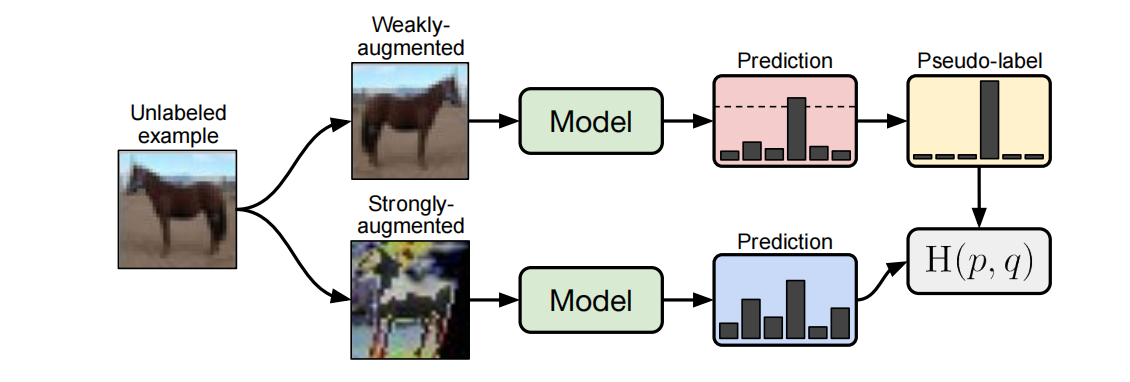

图1. FixMatch框架

那么，为什么可以这么做？为什么weak和strong的预测分布是相近的？于是我们引出FixMatch的2个核心思想：

Consistency regularization

一致性正则化，它有一个很强的假设，就是同一图像经过不同扰动后输入模型，其输出的预测应该是接近或者类似的。故其loss fuction表示为：

$\sum_{b=1}^{\mu B}\Vert p_m(y|\alpha(u_b)) - p_m(y|\alpha(u_b)) \Vert_2^2\tag{1}$

其中$\mu B$代表未标记的数据量，$p_m$是模型，$\alpha$是一个弱扰动(简单的数据增广)。因为数据增广是具有随机性的，所以上式两项上并不一定相同。

Pseudo-labeling

伪标签的思想，是希望利用置信度高的数据进行自我训练，从而提高模型性能，具体而言，体现为下面的损失函数：

$\frac{1}{\mu B}\sum_{b=1}^{\mu B}\Bbb{I}\left(\max(q_b)\geq \tau\right)\text{H}(\hat{q}_b, q_b)\tag{2}$

可以看到，上式设置了一个阈值$\tau$用于控制置信度，只有置信度高于阈值的才进行loss的计算。式子中 $ \hat{q}_b=\arg \max q_b $ ，是指预测分布中分数最高的那个类别，也称为硬标签。

FixMatch结合了这两个思想：即使用弱扰动的图像通过模型生成的伪标签，来监督强扰动的预测结果。具体来说，模型先预测弱扰动图像的分布，并得到硬标签。如果该标签的置信度高于阈值，则将强扰动图像的预测输出和该标签做一个交叉熵损失：

$\begin{aligned} q_b &= p_m(y|\alpha (u_b))\\ \hat{q}_b &= \arg \max q_b\\ \mathcal{L}_u &= \frac{1}{\mu B}\sum_{b=1}^{\mu B}\Bbb{I}\left(\max(q_b)\geq \tau\right)\text{H}(\hat{q}_b, p_m(y|\mathcal{A}(u_b))) \end{aligned}\tag{3}$

其中 $\mathcal{A}(\cdot)$ 就是强扰动(强数据增广)。

最后，数据增广也是FixMatch关键的一环，在原论文中，作者对增广做了如下设置：

弱扰动：标准的flip-and-shift增广，即水平翻转或垂直翻转；

强扰动：作者认为基于强化学习的AutoAugment需要很多带标签的数据，并不适合SSL任务。所以作者采用了以下两个增广方式：

RandAugment：只需要搜索增强操作的数量N和全局的增强幅度M(分为10个等级，10为最强)，代码如下：

# Identity是恒等变换，不做任何增强
transforms = ['Identity', 'AutoContrast', 'Equalize', 'Rotate', 'Solarize', 
              'Color', 'Posterize', 'Contrast', 'Brightness', 'Sharpness', 
              'ShearX', 'ShearY', 'TranslateX', 'TranslateY']

def randaugment(N, M):
"""Generate a set of distortions.
Args:
N: Number of augmentation transformations to apply sequentially.
M: Magnitude for all the transformations.
"""
sampled_ops = np.random.choice(transforms, N)
return [(op, M) for op in sampled_ops]

CTAugment：一种在线学习的方法。该方法先定义一组transforms(如旋转、裁剪等)以及每种变换可能的幅度(旋转的角度等)，然后维护一个变换-幅度-概率表，记录每种变换和幅度的概率，初始化为均匀分布。对于每一张unlabelled图像，从表中随机采样弱增强(变换+幅度)和强增强(变换+幅度)，然后利用弱增强生成伪标签。如果置信度高于阈值则计算伪标签和强增强的预测分布之间的交叉熵损失。最后，根据损失大小更新概率表，损失小，则提高相应概率。

2. UniMatch

UniMatch建立在FixMatch引入图像级强扰动的思想上。直观地说，它的成功在于该模型更有可能对 $x^w$ 产生高置信度和质量的预测，而 $x^s$ 对我们的模型学习更有效，因为强扰动引入了额外的信息，并减轻了确认偏差。具体来说，作者认为FixMatch的强扰动是性能优越的关键(或者说weak-to-strong框架非常优越)。于是作者认为可以进一步发挥强扰动的潜力。它们做了2个方向的改进：

同时探索image和feature两个层面的扰动 - 探索更广泛的扰动空间
Dual-stream 扰动，充分利用预定义的image扰动空间。

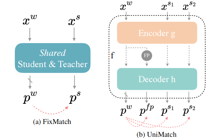
图2. FixMatch和UniMatch对比

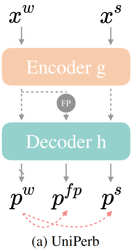
2.1 UniPerb - Perturbations for Images and Features

即同时对image和feature扰动的方法。作者将模型 $f$ 拆成了encoder $g$ 和decoder $h$，$x^w$ 在通过编码器后得到特征，再施加一个特征扰动 $\mathcal{P}$ 得到特征扰动后的新特征 $FP$。这样经过解码器，我们同时可获得(图像)弱扰动的预测分布、特征强扰动的预测分布、(图像)强扰动的预测分布，如下图所示：

图3. UniPerb

使用公式可以表示为：

$\begin{aligned} p^w &= \hat{F}\left(\mathcal{A}^w(x^u) \right);\quad p^s = F\left(\mathcal{A}^s\left(\mathcal{A}^w(x^u)\right) \right)\\ e^w &= g(x^w)\\ p^{fp} &= h\left(\mathcal{P}\left(e^w \right)\right)\\ \mathcal{L}_u &= \frac{1}{B_u}\sum \Bbb{I}\left(\max(p^w)\geq \tau \right)\left(\text{H}(p^w, p^s), \text{H}(p^w, p^{fp}) \right) \end{aligned}\tag{4}$

其中， $x^w$ 是$x^u$经过弱扰动的图像； $\hat F$ 是弱扰动图像的教师模型， $F$ 是强扰动图像使用的学生模型，这里他们俩完全相同。

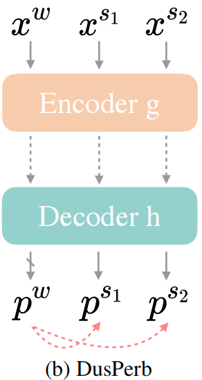
2.2 DusPerb - Dual-Stream Perturbations

作者受到其他工作的影响，认为为无标签图像数据构建多个view作为输入可以更好的利用扰动空间。简单地，他们为一张图像设置2个强扰动视图：$x^{s_1}$和$x^{s_2}$。因为 $\mathcal{A}^s$ 具有随机性，故这两个视图不同。该模式的结构如下图所示：

图4. DusPerb

作者将该结构的优越性归功于 对比学习 (而不是单纯doubled unlabeled batch size)：$x^{s_1}$ 和 $x^{s_2}$ 都应该和 $x^w$ 中预测概率最高的类别接近，等价于 $x^{s_1}$ 和 $x^{s_2}$ 互相接近，这可以使用InfoNCE Loss实现：

论文原文

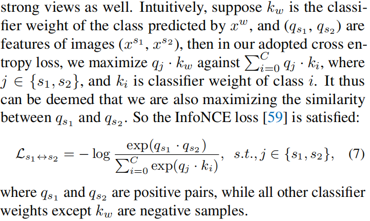
最终模型结合了UniPerb和DusPerb，Loss表示为

$\mathcal{L}_u = \frac{1}{B_u} \sum \Bbb{I}\left(\max(p^w)\geq \tau \right)\cdot \left( \lambda \text{H}(p^w, p^{fp}) + \frac{\mu}{2}\left(\text{H}(p^w, p^{s_1}) + \text{H}(p^w, p^{s_2})\right) \right)\tag{5}$

3. 实验结果和消融研究

由于是新的SOTA，论文在三个数据集上展现出了强劲表现。这里简单摘录在pascal voc 2012数据集上的一些表现(因为下文复现时仅使用该数据集 )。

labelled data数量

图5. 在不同标注数据使用量下，模型在Pascal上的表现

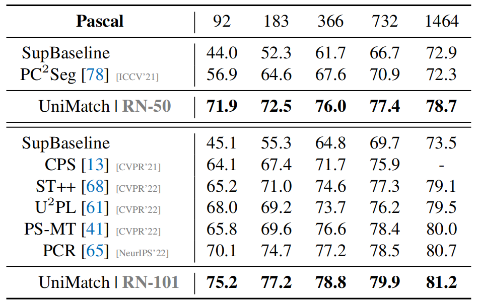
可以看到UniMatch不仅准确率高，还比较稳定，在标注数据较少(如，92)的情况下依然还有较高精度。

labelled data占比

图6. 在不同标注数据占比下，模型在Pascal上的表现

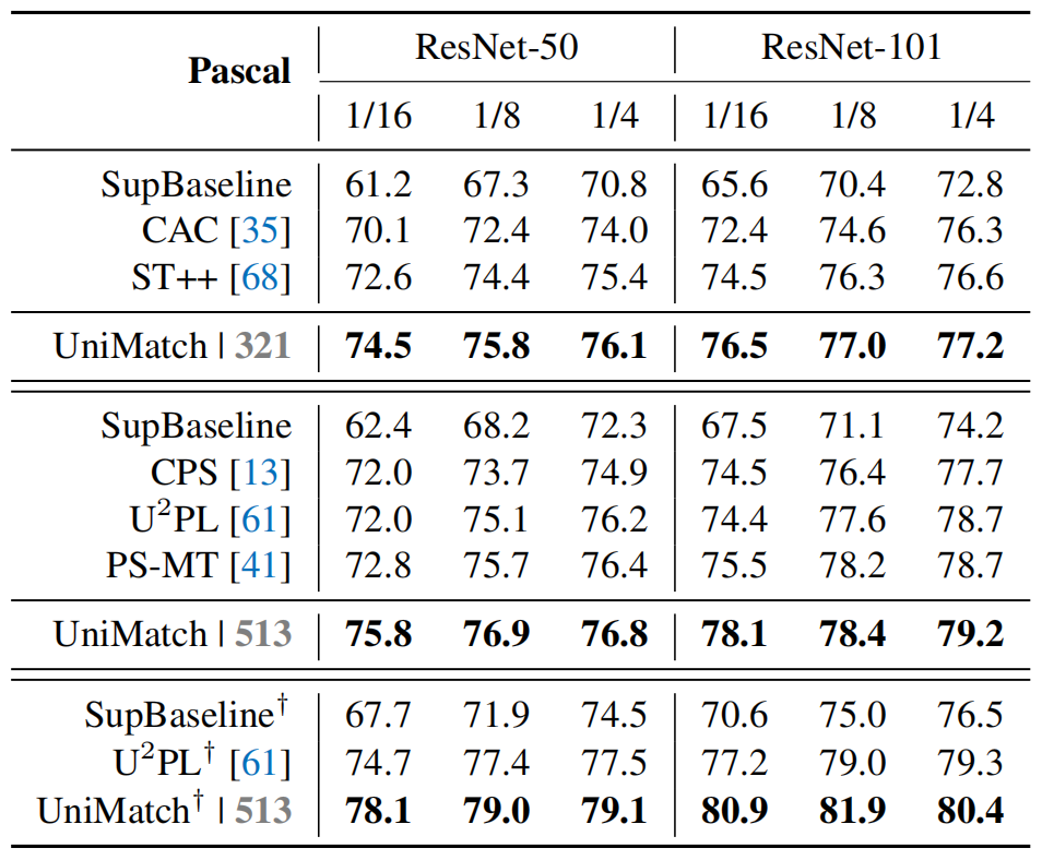
UniMatch在标注数据占比较少(如，1/16)的情况下依然还有较高精度。

消融实验

这一块我们简单列举一下论文的结论：

The improvement of diverse perturbations is non-trivial：即多种类型的强扰动(2×image+feature)是比简单设置3个image强扰动有效的；
The improvement of dual-stream perturbation is non-trivial：论文证明双流扰动的成功不是因为增加了一个batch内的unlabelled data；
The necessity of separating image- and feature-level perturbations into independent streams：即分离不同类型的扰动是有效的；
More perturbation streams：论文证明图像级多流扰动提升有限，双流以已经足够了；

…

实验结果复现

下文分析和修改的代码源自论文仓库： https://github.com/LiheYoung/UniMatch .

1. 下载代码、模型和数据

1.1 代码下载

关于代码的Installation，直接按照默认方法：

cd UniMatch
conda create -n unimatch python=3.10.4
conda activate unimatch
pip install -r requirements.txt # 别急,请先按照下面的第一条修改文件;
pip install torch==1.12.1+cu113 torchvision==0.13.1+cu113 -f https://download.pytorch.org/whl/torch_stable.html

值得强调的是，代码其实包含一些Bug，需要简单处理一下：

在requirements.txt中，需要将sklearn改成scikit-learn，保证pip install 顺利进行；

在unimatch.py中，切记将下面这行代码

1	parser.add_argument('--local_rank', default=0, type=int)

改为

1	parser.add_argument('--local-rank', default=0, type=int)

不然你的local-rank参数不被识别；

如果你是单机单卡或者单机多卡(例如我)，可以将train.sh配置为

export CUDA_VISIBLE_DEVICES=0,1,2,3

python -m torch.distributed.launch \
    --nnodes 1 \
    --nproc_per_node=$1 \
    $method.py \
    --config=$config --labeled-id-path $labeled_id_path --unlabeled-id-path $unlabeled_id_path \
    --save-path $save_path 2>&1 | tee $save_path/$now.log

无需设置port等参数。

1.2 预训练模型下载

预训练的模型在原仓库中有3种：ResNet50/ResNet101/xception，在复现时默认使用resnet101，如果时间允许，我们将尝试其他模型的复现。

1.3 数据集下载

数据集由于时间和资源有限，仅仅复现关于Pascal VOC 2012数据集的一些结果。

Pascal: JPEGImages | SegmentationClass

其他数据集见原仓库。

2. 训练的实现

我们准备好了数据，可以按照下面的算法图完成模型训练：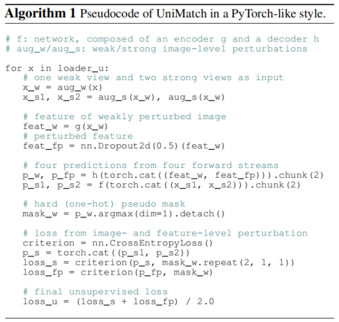

图7. 算法示意图

2.1 数据增广

这里说的数据增广，其实是指strong view的强扰动和weak view的弱扰动。

相关文件：./dataset/semi.py

在图7中指代下面这几行代码：

1
2
3

# one weak view and two strong views as input
x_w = aug_w(x)
x_s1, x_s2 = aug_s(x_w), aug_s(x_w)

源代码在实现这几行时，首先让每一张图像完成弱扰动：

img, mask = resize(img, mask, (0.5, 2.0))
ignore_value = 254 if self.mode == 'train_u' else 255
img, mask = crop(img, mask, self.size, ignore_value)
img, mask = hflip(img, mask, p=0.5)

其中img是RGB图像，mask是分割的掩码。现在，这个经过弱扰动的图像img就是$x^w$，同时，我们将其复制两份，得到$x^{s_1}$和$x^{s_2}$。当然$x^{s_1}$和$x^{s_2}$还需要经过强扰动，成为2个strong view，实现Dual-Stream Perturbations。

1	img_w, img_s1, img_s2 = deepcopy(img), deepcopy(img), deepcopy(img)

进行强扰动的代码(以处理$x^{s_1}$为例)如下：

if random.random() < 0.8:
    # 随机调整亮度、对比度、饱和度和色调
    img_s1 = transforms.ColorJitter(0.5, 0.5, 0.5, 0.25)(img_s1)
img_s1 = transforms.RandomGrayscale(p=0.2)(img_s1)  # 随机灰度化
img_s1 = blur(img_s1, p=0.5)    # 随机模糊
cutmix_box1 = obtain_cutmix_box(img_s1.size[0], p=0.5)  # 随机获取CutMix的区域

因为这些数据增强方法设置了概率，故不同的epoch或者是$x^{s_1}$和$x^{s_2}$之间，增强的效果都是不同的。其中我对于CutMix操作还比较好奇，去查看了函数定义。发现CutMix就是mask掉一块区域(该区域的宽高和位置都是一定程度随机的)，然后用其他图片中相同位置的区域来填充。

由于Pascal数据集的标注图像mask中包含254这个无效像素值，没有对应类别，作者使用ignore_mask忽略它：

ignore_mask = Image.fromarray(np.zeros((mask.size[1], mask.size[0])))

img_s1, ignore_mask = normalize(img_s1, ignore_mask)
img_s2 = normalize(img_s2)

mask = torch.from_numpy(np.array(mask)).long()
ignore_mask[mask == 254] = 255

取值为255是因为crop操作对哪些裁剪时遇到的padding都设置值为255，同样也是无效区域，这里相当于合并了。于是，经过图像增广等操作后，我们的输入数据可能就包含以下几个部分：

$x^w$: 即img_w，在return时还需要normalize一下；
$x^{s_1}$: 即img_s1，经过强扰动，且已经normalize；
$x^{s_2}$: 即img_s2，经过强扰动，且已经normalize；
ignore_mask: 用于忽略无效的像素；
cutmix_box1: 从$x^{s_1}$获取的mask掉的CutMix区域；
cutmix_box2: 从$x^{s_2}$获取的mask掉的CutMix区域；

了解增广的细节后，我们可以构建3个数据集，分别是有标签监督数据、无标签数据、和验证数据：

trainset_u = SemiDataset(cfg['dataset'], cfg['data_root'], 'train_u',
                         cfg['crop_size'], args.unlabeled_id_path)
trainset_l = SemiDataset(cfg['dataset'], cfg['data_root'], 'train_l',
                         cfg['crop_size'], args.labeled_id_path, 
                         nsample=len(trainset_u.ids))
valset = SemiDataset(cfg['dataset'], cfg['data_root'], 'val')

将它们分别转为Dataloader后，通过下面的代码进行分批训练：

loader = zip(trainloader_l, trainloader_u, trainloader_u)

for i, ((img_x, mask_x),
        (img_u_w, img_u_s1, img_u_s2, ignore_mask, cutmix_box1, cutmix_box2),
        (img_u_w_mix, img_u_s1_mix, img_u_s2_mix, ignore_mask_mix, _, _)) 
        in enumerate(loader):

接下来的分析，都在上述循环中，请关注从loader中取出的这些数据！

填充CutMix

最后一步，将cutmix操作完成，具体来说，我们用第二个trainloader_u中获取的数据来填充我们的$s_1$和$s_2$：

img_u_s1[cutmix_box1.unsqueeze(1).expand(img_u_s1.shape) == 1] = \
    img_u_s1_mix[cutmix_box1.unsqueeze(1).expand(img_u_s1.shape) == 1]

img_u_s2[cutmix_box2.unsqueeze(1).expand(img_u_s2.shape) == 1] = \
    img_u_s2_mix[cutmix_box2.unsqueeze(1).expand(img_u_s2.shape) == 1]

2.2 模型预测

在图7中，这部分表示为：

# feature of weakly perturbed image
feat_w = g(x_w)
# perturbed feature
feat_fp = nn.Dropout2d(0.5)(feat_w)
# four predictions from four forward streams
p_w, p_fp = h(torch.cat((feat_w, feat_fp))).chunk(2)
p_s1, p_s2 = f(torch.cat((x_s1, x_s2))).chunk(2)

在unimatch.py中，并没有展现出将$f$拆分为 $h(g(x))$ 的细节，而是直接通过model生成预测，所以dropout2d应该包含在model里了。我们截取了下面代码，作为上述部分的实现，并提供解释：

num_lb, num_ulb = img_x.shape[0], img_u_w.shape[0]

# img_x是带标签的监督图像数据，通过计算pred_x可以进行有监督训练.
preds, preds_fp = model(torch.cat((img_x, img_u_w)), True)  # need_fp=True,进行dropout
pred_x, pred_u_w = preds.split([num_lb, num_ulb])   # pred_u_w => p_w
pred_u_w_fp = preds_fp[num_lb:] # pred_u_w_fp => p_fp,进行特征层面的自监督训练

# pred_u_s1 => p_s1, pred_u_s2 => p_s2
pred_u_s1, pred_u_s2 = model(torch.cat((img_u_s1, img_u_s2))).chunk(2)

2.3 Loss计算

在图7中指代一下部分：

# hard (one-hot) pseudo mask
mask_w = p_w.argmax(dim=1).detach()
# loss from image- and feature-level perturbation
criterion = nn.CrossEntropyLoss()
p_s = torch.cat((p_s1, p_s2))
loss_s = criterion(p_s, mask_w.repeat(2, 1, 1))
loss_fp = criterion(p_fp, mask_w)
# final unsupervised loss
loss_u = (loss_s + loss_fp) / 2.0

由于$x^{s_1}$和$x^{s_2}$进行过CutMix，而$x^{w}$并没有做这些强扰动，所以想得到无标签自监督的标签mask_w很复杂，因此损失的计算并不简单。我们基于现有参数逐步分析：

首先，对于用来填充cutmix的数据img_u_w_mix，我们利用模型预测其分割结果mask_u_w_mix；同时，$x^w$也通过模型获得了pred_u_w(见2.2)，我们同样可以获得mask_u_w：

with torch.no_grad():
    model.eval()

    pred_u_w_mix = model(img_u_w_mix).detach()
    conf_u_w_mix = pred_u_w_mix.softmax(dim=1).max(dim=1)[0]
    mask_u_w_mix = pred_u_w_mix.argmax(dim=1)

...

model.train()

...

pred_u_w = pred_u_w.detach()
conf_u_w = pred_u_w.softmax(dim=1).max(dim=1)[0]
mask_u_w = pred_u_w.argmax(dim=1)

由于我们知道了$s_1$和$s_2$CutMix框的位置，所以我们直接将上面的两个图像的mask结合，就可以得到自监督label：

# 由于cutmix框不一样，这里分别获得cutmixed1和cutmixed2的mask及其conf等
mask_u_w_cutmixed1, conf_u_w_cutmixed1, ignore_mask_cutmixed1 = \
    mask_u_w.clone(), conf_u_w.clone(), ignore_mask.clone()
mask_u_w_cutmixed2, conf_u_w_cutmixed2, ignore_mask_cutmixed2 = \
    mask_u_w.clone(), conf_u_w.clone(), ignore_mask.clone()

mask_u_w_cutmixed1[cutmix_box1 == 1] = mask_u_w_mix[cutmix_box1 == 1]
conf_u_w_cutmixed1[cutmix_box1 == 1] = conf_u_w_mix[cutmix_box1 == 1]
ignore_mask_cutmixed1[cutmix_box1 == 1] = ignore_mask_mix[cutmix_box1 == 1]

mask_u_w_cutmixed2[cutmix_box2 == 1] = mask_u_w_mix[cutmix_box2 == 1]
conf_u_w_cutmixed2[cutmix_box2 == 1] = conf_u_w_mix[cutmix_box2 == 1]
ignore_mask_cutmixed2[cutmix_box2 == 1] = ignore_mask_mix[cutmix_box2 == 1]

最后，我们给出4个损失：

第一个损失：有监督损失。使用img_x的预测结果pred_x和标签mask_x计算：

1	loss_x = criterion_l(pred_x, mask_x)

第二&三个损失：图像层面自监督损失。通过$s_1$和$s_2$的预测结果及其对应label计算：

loss_u_s1 = criterion_u(pred_u_s1, mask_u_w_cutmixed1)
loss_u_s1 = loss_u_s1 * (
    (conf_u_w_cutmixed1 >= cfg['conf_thresh']) & (ignore_mask_cutmixed1 != 255))
loss_u_s1 = loss_u_s1.sum() / (ignore_mask_cutmixed1 != 255).sum().item()

loss_u_s2 = criterion_u(pred_u_s2, mask_u_w_cutmixed2)
loss_u_s2 = loss_u_s2 * (
    (conf_u_w_cutmixed2 >= cfg['conf_thresh']) & (ignore_mask_cutmixed2 != 255))
loss_u_s2 = loss_u_s2.sum() / (ignore_mask_cutmixed2 != 255).sum().item()

第四个损失：特征层面的自监督损失。通过$x^{fp}$的预测结果pred_u_w_fp和$x^w$的预测结果计算：

1
2
3

loss_u_w_fp = criterion_u(pred_u_w_fp, mask_u_w)
loss_u_w_fp = loss_u_w_fp * ((conf_u_w >= cfg['conf_thresh']) & (ignore_mask != 255))
loss_u_w_fp = loss_u_w_fp.sum() / (ignore_mask != 255).sum().item()

Total

1	loss = (loss_x + loss_u_s1 * 0.25 + loss_u_s2 * 0.25 + loss_u_w_fp * 0.5) / 2.0

3. 模型结构解析

模型结构在本文中显然是Encoder-Decoder架构，具体而言，我们进行如下分析：

3.1 Encoder

该论文的Encoder设置为ResNet和xception，为了便于讨论，只以ResNet101为例。这里不再展示模型的结构，直接看它的forward：

def base_forward(self, x):
    x = self.conv1(x)       # (3, 224, 224) => (128, 112, 112)
    x = self.bn1(x)
    x = self.relu(x)
    x = self.maxpool(x)     # (128, 112, 112) => (128, 56, 56)

    c1 = self.layer1(x)     # 3个Bottleneck, (128, 56， 56) => (64*4, 56, 56)
    c2 = self.layer2(c1)    # 4个Bottleneck, stride=2, (256, 56, 56) => (128*4, 28, 28)
    c3 = self.layer3(c2)    # 23个Bottleneck, stride=2, (512, 28, 28) => (256*4, 14, 14)
    c4 = self.layer4(c3)    # 3个Bottleneck, stride=2, (1024, 14, 14) => (512*4, 7, 7)

    return c1, c2, c3, c4

我们以一张大小为(3,224,224)的图片为例，相关提示已经在上面的注释中。通过resnet，我们已得到两种视角的特征：c1和c4。

3.2 Decoder

首先介绍Decoder的一个模块ASPPModule，由ASPPConv和ASPPPooling等组合而成。

ASPPConv引入了空洞卷积，其维度计算公式为：

1 2	H_out = (H_in + 2 * padding - dilation * (kernel_size - 1) - 1) / stride + 1 W_out = (W_in + 2 * padding - dilation * (kernel_size - 1) - 1) / stride + 1

其实现代码如下：

def ASPPConv(in_channels, out_channels, atrous_rate):
    block = nn.Sequential(nn.Conv2d(in_channels, out_channels, 3, padding=atrous_rate,
                                    dilation=atrous_rate, bias=False),
                          nn.BatchNorm2d(out_channels),
                          nn.ReLU(True))
    return block

ASPPPooling的代码为：

class ASPPPooling(nn.Module):
    def __init__(self, in_channels, out_channels):
        super(ASPPPooling, self).__init__()
        self.gap = nn.Sequential(nn.AdaptiveAvgPool2d(1),
                                 nn.Conv2d(in_channels, out_channels, 1, bias=False),
                                 nn.BatchNorm2d(out_channels),
                                 nn.ReLU(True))

    def forward(self, x):
        h, w = x.shape[-2:]
        pool = self.gap(x)
        return F.interpolate(pool, (h, w), mode="bilinear", align_corners=True)

举例而言，数据维度经过如下变化：

设 x.size = (2048, 7, 7)
|__nn.AdaptiveAvgPool2d(1) =>  (2048, 1, 1)
|__nn.Conv2d(2048, 256, 1, bias=False) => (256, 1, 1)
|__nn.BatchNorm2d(out_channels) => (256, 1, 1)
|__nn.ReLU(True) => (256, 1, 1)
|__F.interpolate => (256, 7, 7)     # 插值

最后，ASPPModule通过这些模块组合而成，代码为：

class ASPPModule(nn.Module):
    def __init__(self, in_channels, atrous_rates):
        super(ASPPModule, self).__init__()
        out_channels = in_channels // 8
        rate1, rate2, rate3 = atrous_rates

        self.b0 = nn.Sequential(nn.Conv2d(in_channels, out_channels, 1, bias=False),
                                nn.BatchNorm2d(out_channels),
                                nn.ReLU(True))
        self.b1 = ASPPConv(in_channels, out_channels, rate1)
        self.b2 = ASPPConv(in_channels, out_channels, rate2)
        self.b3 = ASPPConv(in_channels, out_channels, rate3)
        self.b4 = ASPPPooling(in_channels, out_channels)

        self.project = nn.Sequential(nn.Conv2d(5 * out_channels, out_channels,
                                               1, bias=False),
                                     nn.BatchNorm2d(out_channels),
                                     nn.ReLU(True))

    def forward(self, x):
        feat0 = self.b0(x)
        feat1 = self.b1(x)
        feat2 = self.b2(x)
        feat3 = self.b3(x)
        feat4 = self.b4(x)
        y = torch.cat((feat0, feat1, feat2, feat3, feat4), 1)
        return self.project(y)

经过该模块的数据，例如(2048,7,7)，最终变为(256, 7, 7)。Decoder的具体实现见3.3.

3.3 Total model

我们将分析写成了注释，添加在下面的代码中：

class DeepLabV3Plus(nn.Module):
    def __init__(self, cfg):
        super(DeepLabV3Plus, self).__init__()
        # Encoder,默认为resnet101
        if 'resnet' in cfg['backbone']:
            self.backbone = resnet.__dict__[cfg['backbone']](
                pretrained=True, 
                replace_stride_with_dilation=cfg['replace_stride_with_dilation'])
        else:
            assert cfg['backbone'] == 'xception'
            self.backbone = xception(pretrained=True)

        low_channels = 256      # 经过self.head后的通道数,即ASPPModule.out_channels
        high_channels = 2048    # 经过resnet后的c4的通道数

        # cfg['dilations'] = [6, 12, 18],提供了不同感受野的信息,并经过融合。
        self.head = ASPPModule(high_channels, cfg['dilations'])

        # 减少c1的通道数，256 => 48, 浓缩信息+减少参数量
        self.reduce = nn.Sequential(nn.Conv2d(low_channels, 48, 1, bias=False),
                                    nn.BatchNorm2d(48),
                                    nn.ReLU(True))

        # 融合c1(低级信息)和c4(高级信息)的信息,强制输出维度为256
        self.fuse = nn.Sequential(nn.Conv2d(high_channels // 8 + 48, 256, 3, 
                                            padding=1, bias=False),
                                  nn.BatchNorm2d(256),
                                  nn.ReLU(True),
                                  nn.Conv2d(256, 256, 3, padding=1, bias=False),
                                  nn.BatchNorm2d(256),
                                  nn.ReLU(True))

        self.classifier = nn.Conv2d(256, cfg['nclass'], 1, bias=True)

    def forward(self, x, need_fp=False):
        """ 
        设x.size = (2,3,224,224), need_fp=True,模拟将s1,s2这2个数据cat后进入模型
        """
        h, w = x.shape[-2:]     # h=224,w=224

        feats = self.backbone.base_forward(x)   # 获得4种特征图c1~c4
        c1, c4 = feats[0], feats[-1]            # c1=(2,256,56,56),c4=(2,2048,7,7)

        if need_fp:
            # 这里nn.Dropout2d(0.5)就是构建fp
            # 这里做了一些拼接,例如
            # torch.cat((c1, nn.Dropout2d(0.5)(c1))).size = (4,256,56,56)
            # torch.cat((c4, nn.Dropout2d(0.5)(c4))).size = (4,2048,7,7)
            outs = self._decode(torch.cat((c1, nn.Dropout2d(0.5)(c1))),
                                torch.cat((c4, nn.Dropout2d(0.5)(c4))))
            # outs.size = (4,21,56,56),注意这是因为self.classifier将channel设为class数21
            outs = F.interpolate(outs, size=(h, w), mode="bilinear", align_corners=True)
            # out和out_fp分别代表x_w和经过特征扰动后的fp的输出
            out, out_fp = outs.chunk(2)    

            return out, out_fp

        out = self._decode(c1, c4)      # out.size = (2,21,56,56)
        out = F.interpolate(out, size=(h, w), mode="bilinear", align_corners=True)
        # # out.size = (2,21,224,224)
        return out

    def _decode(self, c1, c4):
        """ 设c1.size=(256,56,56), c4.size=(2048,7,7), 详见resnet """
        c4 = self.head(c4)      # c4: (2048,7,7) => (256,7,7)
        # c4: (256,7,7) => (256,56,56)
        c4 = F.interpolate(c4, size=c1.shape[-2:], mode="bilinear", align_corners=True)

        c1 = self.reduce(c1)    # c1: (256,56,56) => (48,56,56)

        feature = torch.cat([c1, c4], dim=1)    # feature.size=(256+48,56,56)
        feature = self.fuse(feature)            # => feature.size=(256,56,56)

        out = self.classifier(feature)          # 像素级分类，out=(21,56,56)

        return out

4. 复现结果

由于时间仓促，目前只复现了backbone为ResNet101在数据集Pascal上的表现，如下表所示:

Pascal / UniMatch \| ResNet101	92	183	366	732	1464
Paper	75.2	77.2	78.8	79.9	81.2
OurWork	75.2	76.8	78.5	79.2	80.8

Pascal / UniMatch \| ResNet101	1/16	1/8	1/4
Paper \| 321	76.5	77.0	77.2
OurWork \| 321	76.6	77.4	77.4

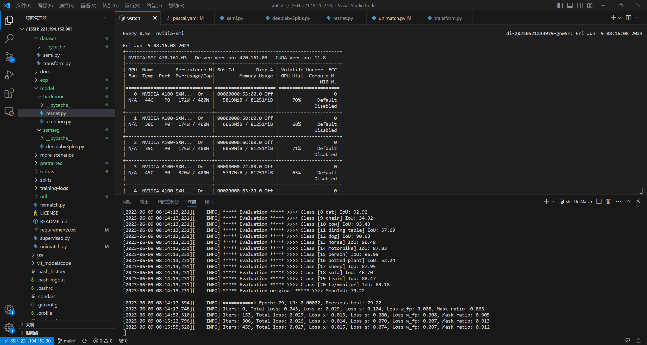
我们的复现基本接近或者达到论文中的精度，证明有效。我们展示两张复现时的截图，可供参考：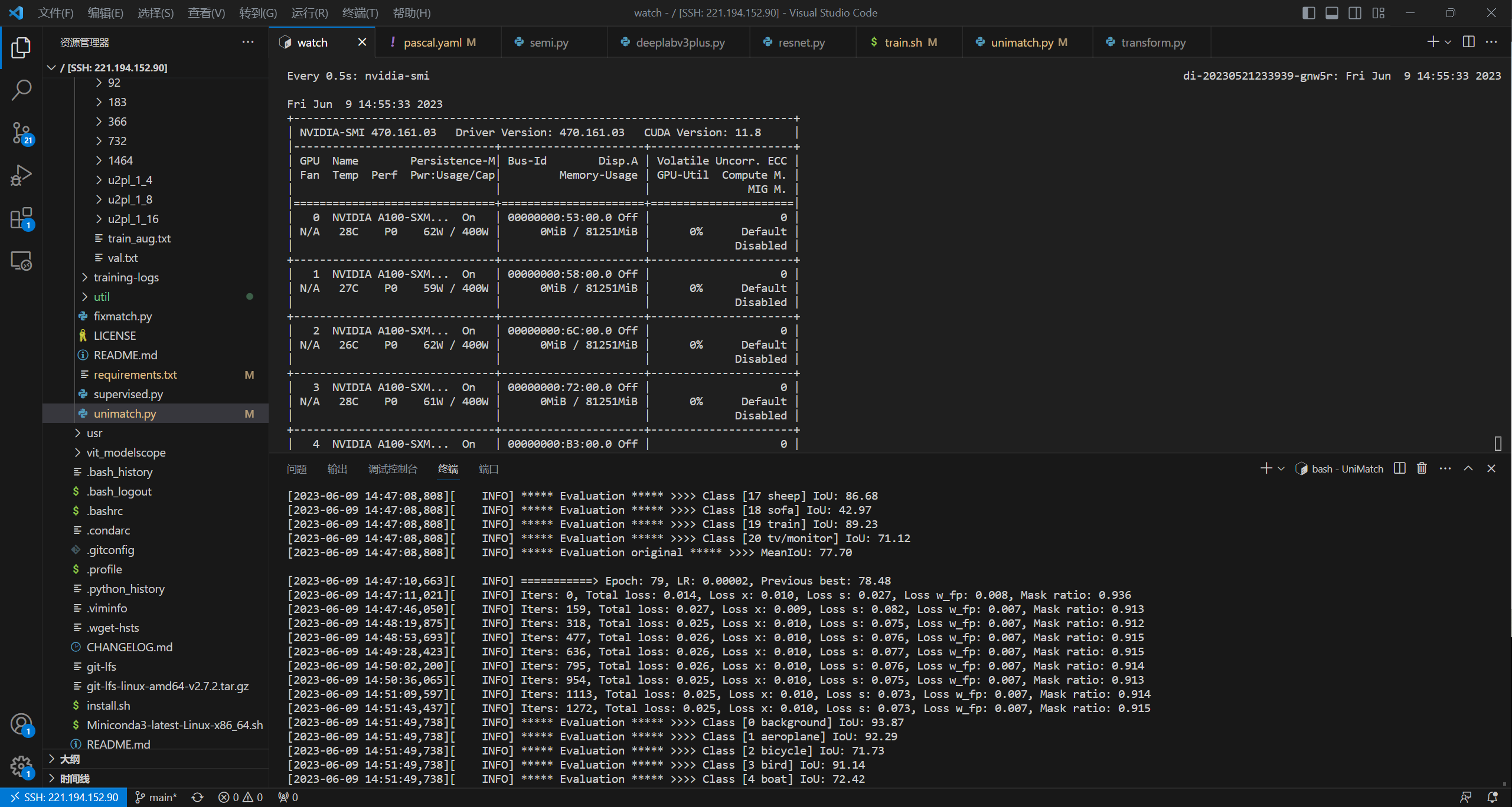

图8. resnet101 | pascal-366

图8. resnet101 | pascal-732

3. 基于FlexMatch的改进

由于作者认为FixMatch足够强大、足够简单，所以以其为baseline。我们尝试使用FlexMatch方法为baseline设计一个类似的UniMatch模型。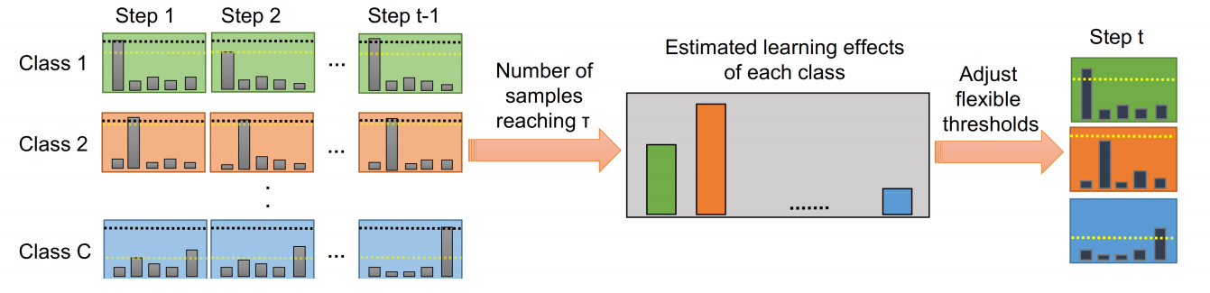

图9. FlexMatch阈值调整方法

FlexMatch方法，就是将下式固定的 $\tau$ 转化为可以动态调整的形式，但又不显示引入参数：

$\mathcal{L}_u = \frac{1}{\mu B}\sum_{b=1}^{\mu B}\Bbb{I}\left(\max(q_b)\geq \tau\right)\text{H}(\hat{q}_b, p_m(y|\mathcal{A}(u_b)))\tag{6}$

这种动态调整方法被称为Curriculum Pseudo Labeling (CPL)方法。

FlexMatch认为一个类别预测的置信度越低，说明对该类的学习仍不够充分，应该降低阈值鼓励学习，即阈值和类别的学习效果有关。论文中使用预测属于该类且置信度大于阈值的无标签数据数量衡量一个类别的学习效果：

$\sigma_{t}(c) = \sum_{n=1}^{N}\Bbb{I}\left(\max(p_{m,t}(y|u_n))\geq \tau\right)\Bbb{I}\left(\arg \max(p_{m,t}(y|u_n)) = c \right)\tag{7}$

</a>

其中 $t$ 是指step t时刻。我们将上式得到的学习效果 $\sigma_{t}(c)$ 归一化，得到step t时每个类别的阈值：

$\beta_t(c) = \frac{\sigma_t(c)}{\max_{c} \sigma_t} \tag{8}$

</a>

$\mathcal{T}_t(c) = \beta_t(c)\cdot\tau\tag{9}$

</a>

实际上这个动态阈值$\mathcal{T}_t(c)$还会施加一个非线性函数：

$\mathcal{T}_t(c) = \mathcal{M}\left(\beta_t(c)\right)\cdot \tau\tag{10}$

最后损失函数修改为：

$\mathcal{L}_{u,t} = \frac{1}{\mu B}\sum_{b=1}^{\mu B}\Bbb{I}\left(\max(q_b)\geq \mathcal{T}_t(\arg \max q_b) \right)\text{H}(\hat{q}_b, p_m(y|\mathcal{A}(u_b)))\tag{11}$

1. 改进的代码

通过调研TorchSSL代码库，我们可以对FlexMatch方法有更清晰的认识。我们考虑在fixmatch.py和unimatch.py上修改代码，加入动态阈值。

1.1 fixmatch.py

在每一轮开始之前，我们要预定义2个变量：

selected_label：一个存储分类情况的变量。在flexmatch的源码实现中，该参数将记录所有未标记图片的类别硬标签。但在语义分割任务中，一张图片的类别标签大小为(W,H)，一旦图像数量较大则会导致空间占用较多、运行速度变慢，所以这里采用一个队列queue来实现它。当队列已满时，将最早进入队列的batch移除，将新的batch移入。默认的队列长度queue_length为batch_size的100倍。
classwise_acc：记录每个类别的学习情况，即公式(7)的$\sigma_t(c)$。

# selected_label.size = (N,W,H),记录每个像素的类别
# classwise_acc.size = (C,), 记录每个类别的准确率
queue_length = cfg["batch_size"] * cfg["queue_num"]     # 记录队列总长度
head_length = cfg["batch_size"]                         # 记录队列的头
selected_label = torch.ones(
    (queue_length, cfg["crop_size"], cfg["crop_size"]), dtype=torch.long
    ) * cfg["nclass"]
selected_label = selected_label.cuda().detach()
classwise_acc = torch.zeros((cfg["nclass"],)).cuda()

在每一个step计算loss之前，我们需要根据式(8)得到归一化值。

1
2
3

pseudo_counter = torch.bincount(selected_label.reshape(-1)) # 各类别预测数量
if max(pseudo_counter) < selected_label.shape[0] * (cfg["crop_size"] ** 2):
    classwise_acc = pseudo_counter[:cfg["nclass"]] / max(pseudo_counter)

接着我们根据式(9,10)可以得到动态阈值，并以此计算loss：

# u_w_cutmixed_thresh为动态阈值
u_w_cutmixed_thresh = torch.nn.functional.one_hot(
    mask_u_w_cutmixed, num_classes=cfg["nclass"]).to(torch.float)
# u_w_cutmixed_thresh.size = (B,W,H,C)
u_w_cutmixed_thresh =  torch.matmul(u_w_cutmixed_thresh, classwise_acc)  # size=(B,W,H)
u_w_cutmixed_thresh = 0.95 * u_w_cutmixed_thresh / (2. - u_w_cutmixed_thresh)

# mask_u_w_cutmixed是硬标签(B,W,H)，pred_u_s是软标签(B,C,W,H)
loss_u_s = criterion_u(pred_u_s, mask_u_w_cutmixed)     
loss_u_s = loss_u_s * ((conf_u_w_cutmixed - u_w_cutmixed_thresh >= 0) & \
                                       (ignore_mask_cutmixed != 255))
loss_u_s = loss_u_s.sum() / (ignore_mask_cutmixed != 255).sum().item()

# 更新selected_label
select = (conf_u_w_cutmixed >= cfg['conf_thresh']).long()
for k in range(select.shape[0]):
    selected_label[head_length-cfg["batch_size"]:head_length][k][select[k] == 1] =\
                                                mask_u_w_cutmixed[k][select[k] == 1]

一个batch的阈值矩阵大小为(B,W,H)，我们使用one-hot编码使其可以直接与classwise_acc相乘。在计算完loss之后，我们要更新selected_label(记录队列中图像的语义分割标签)，以供下一个step使用。一般我们只需要更新队列末尾的那个batch即可。

最后，我们需要代码来完成队列的push和pop，以实现动态的变化：

new_batch_data = cfg["nclass"] * torch.ones(
    (cfg["batch_size"], cfg["crop_size"], cfg["crop_size"]), dtype=torch.long).cuda()
if head_length < queue_length:
    head_length += cfg["batch_size"]    # 添加新数据
else:
    selected_label[:-cfg["batch_size"]] = selected_label.clone()[cfg["batch_size"]:]
    selected_label[-cfg["batch_size"]:] = new_batch_data

2. 简单的实验验证

由于时间比较局促，目前只验证了model=ResNet101，dataset=Pascal中的部分实验：

实验1：在crop=321的情况下：

Pascal / ResNet101	92	183	366	732	1464
Paper - UniMatch	75.2	77.2	78.8	79.9	81.2
OurWork - FlexUniMatch	/	73.9	76.2	78.5	/

实验2：FixMatch vs. FlexMatch

目前只测试了一组数据，在pascal-crop_321-732-resnet101的设置下，结果为76.79，与FixMatch的对应值77.8还有不小的差距。

3. 一些实验感悟与未来探讨

很遗憾，在实验中并没有把FlexMatch方法做到与FixMatch方法接近。其中loss_u和loss_fp损失依然较大，没能下降到原有水平。

我对造成这个问题的原因的进行了简单分析：

我们为了提高效率选择了使用一个队列，损失了较多数据的信息，队列中的类别可能不能反映整体数据分布；
我们还没有对类别分布展开分析，如果每一个step的类别分布不均衡的话会影响效果；
我们没有调整任何超参数(即，和UniMatch完全一致)，可能会导致lr等不合适的情况；
我们没有修改扰动的组合，也没有尝试验证特征扰动和多流扰动的其他可能；
尽管FlexMatch并没有显式增加参数，但由于对于动态阈值调整的变量$\beta_t(c)$涉及到全部数据的类别信息、以及非线性函数的选择，在语义分割的像素级分类上应用并不简单。

不过，我们也发现增加队列的长度对提升模型效果有一定帮助，但效果增长有限。